Linear Algebra II

November 20, 2014

Lecture 28-29

Filed under: 2014 Fall — hkuyklau @ 8:59 PM

Today we learnt: Every linear operator ${T}$ on inner product space has a “mate” ${T^*}$ such that ${T}$ and ${T^*}$ are related by

$\displaystyle \langle T(v), w\rangle = \langle v, T^*(w)\rangle$ ${\forall}$ ${v,w\in V}$ .

How is ${T^*}$ defined? In today’s lecture we studied the definition of ${T^*}$ , which is based on the important result: If ${f:V\rightarrow {\mathbb R}}$ is a linear transformation, then there exists unique ${z\in V}$ such that ${f(v)=\langle v,z\rangle}$ .

${M_{\mathcal{B}}(T^*) = M_{\mathcal{B}}(T)^T}$ where ${\mathcal{B}}$ is an orthonormal basis for ${V}$ .
This result tells the relation between the matrix representations of ${T}$ and ${T^*}$ w.r.t. orthonormal bases.
If ${T=T^*}$ , then ${M_{\mathcal{B}}(T)}$ is symmetric.
Below we shall see that self-adjoint operator ${T}$ (i.e. satisfying ${T=T^*}$ ) are particularly nice.

Recall that for linear operators on vector spaces, we study the concept of similarity and diagonalization: let us review a few important points below. By definition, “ ${A}$ is similar to ${B}$ ” means ${P^{-1}AP=B}$ for some invertible matrix ${P}$ .

If ${T:V\rightarrow V}$ is a linear operator on vector space (not necessarily inner product space), then ${M_E(T)}$ is similar to ${M_F(T)}$ for any ordered bases ${E}$ and ${F}$ .
If ${A}$ is similar to ${B}$ , then ${A}$ and ${B}$ are matrix representations of the same linear operator.

Next suppose ${A}$ is similar to a diagonal matrix ${D}$ (i.e. ${P^{-1}A P= D}$ ). Write ${P=\begin{pmatrix} \underline{x}_1 & \underline{x}_2 & \cdots & \underline{x}_n\end{pmatrix}}$ and ${D={\rm diag}(\lambda_1, \lambda_2,\cdots, \lambda_n)}$ , then from ${P^{-1} AP=D}$ , we get ${AP=PD}$ , i.e.

$\displaystyle \begin{array}{rcl} && A \begin{pmatrix} \underline{x}_1 & \underline{x}_2 & \cdots & \underline{x}_n\end{pmatrix} = \begin{pmatrix} \underline{x}_1 & \underline{x}_2 & \cdots & \underline{x}_n\end{pmatrix}\begin{pmatrix} \lambda_1 & & & \\ & \lambda_2 & & \\ & & \ddots & \\ & & & \lambda_n\end{pmatrix}\vspace{1mm}\\ \Rightarrow && \begin{pmatrix} A\underline{x}_1 & A\underline{x}_2 & \cdots & A\underline{x}_n\end{pmatrix} = \begin{pmatrix} \lambda_1\underline{x}_1 & \lambda_2\underline{x}_2 & \cdots & \lambda_n\underline{x}_n\end{pmatrix}\vspace{3mm}\\ \Rightarrow && A\underline{x}_i = \lambda_i \underline{x}_i, \quad {i=1,\cdots, n}. \end{array}$

That means ${\lambda_i}$ is the eigenvalue and ${\underline{x}_i}$ is the corresponding eigenvector. Also, ${P}$ is invertible if and only if ${\underline{x}_1,\cdots, \underline{x}_n}$ form a basis for ${{\mathbb R}^n}$ . The converse is also true: when we diagonalize a matrix ${A}$ (assuming ${A}$ is diagonalizable), how do we find ${P}$ and ${D}$ ? We calculate the eigenvalues to get ${D}$ and then calculate the eigenvectors to get ${P}$ .

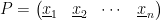
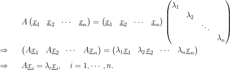
Furthermore, we can present the above result in the setting of linear transformation: Suppose ${P^{-1}A P=D}$ where ${P=\begin{pmatrix} \underline{x}_1 & \underline{x}_2 & \cdots & \underline{x}_n\end{pmatrix}}$ and ${D={\rm diag}(\lambda_1, \lambda_2,\cdots, \lambda_n)}$ . Then the linear operator ${T_A:{\mathbb R}^n\rightarrow {\mathbb R}^n}$ , ${T_A(\underline{v})= A\underline{v}}$ has the standard matrix representation ${M_{St}(T_A)= A}$ . If we set ${\mathcal{E}=[\underline{x}_1,\cdots, \underline{x}_n]}$ (the ordered basis consisting of eigenvectors), then ${M_{\mathcal{E}}(T_A)= D}$ is diagonal. Using this viewpoint, we have another description (or criterion) for diagonalizable matrices:

The matrix ${A}$ is similar to a diagonal matrix
${\Leftrightarrow}$ There exists a basis ${\mathcal{E}}$ for ${{\mathbb R}^n}$ such that ${M_{\mathcal{E}}(T_A)}$ is diagonal
${\Leftrightarrow}$ There exists a basis ${\mathcal{E}=[\underline{x}_1,\cdots, \underline{x}_n]}$ for ${{\mathbb R}^n}$ such that ${T_A(\underline{x}_i)=\lambda_i \underline{x}_i}$ , ${i=1,\cdots, n}$
${\Leftrightarrow}$ We can find a basis ${\mathcal{E}}$ consisting of eigenvectors of ${A}$ for ${{\mathbb R}^n}$

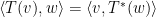
Now we turn back to inner product spaces. If ${V}$ is an inner product space, then we can consider more special basis — orthonormal basis (which are much more convenient, at least from the angle of computation). Hence we may consider the following question in the above diagoanlization problem:

${(**)}$ Can we find an orthonormal basis ${\mathcal{B}}$ such that ${M_{\mathcal{B}}(T_A)}$ is diagonal?

In terms of matrices, this is equivalent to finding a set of orthonormal eigenvectors ${\underline{x}_1,\cdots, \underline{x}_n}$ such that ${P=\begin{pmatrix} \underline{x}_1 & \underline{x}_2 & \cdots & \underline{x}_n\end{pmatrix}}$ such that ${P^{-1}A P= D}$ .

Here we make a nice observation: if ${P=\begin{pmatrix} \underline{x}_1 & \underline{x}_2 & \cdots & \underline{x}_n\end{pmatrix}}$ where ${\langle \underline{x}_i, \underline{x}_j\rangle =1}$ for ${i=j}$ and ${0}$ for ${i\neq j}$ , then

$\displaystyle P^TP=PP^T=I.$

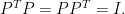
Such a matrix is called an orthogonal matrix (i.e. ${A}$ is orthogonal if ${A^TA=I}$ . Note that ${A^TA=I}$ ${\Rightarrow}$ ${AA^T=I}$ .)

Hence for our problem ${(**)}$ the condition ${P^{-1}AP=D}$ can be rephrased as ${P^T AP=D}$ . That’s why we invoke the concept of orthogonally diagonalizable.

Now we can state the following key result for self-adjoint linear operators (or in matrix setting, symmetric matrices):

Every ${n\times n}$ symmetric matrix ${A}$ has a set of orthonormal eigenvectors which form a basis for ${{\mathbb R}^n}$ .

In the setting of linear operators, every self-adjoint operator ${T:V\rightarrow V}$ (on inner product space) has a set of orthonormal eigenvectors which form a basis for ${V}$ .

See also Lect28-29.pdf in the folder slides.

Leave a Comment

November 10, 2014

Lecture 25

Filed under: 2014 Fall — hkuyklau @ 5:40 PM

We started inner product spaces and finished Section 10.1, covering some basic structures (see Lect25.pdf). More important (and deep) results, as listed below, will come up.

Orthonormal basis and Gram-Schmidt process
Orthogonal complement and Projection
The adjoint of a linear operator (on inner product space)
Orthogonal diagonalization and Principal axis theorem
Orthogonal similarity and Schur’s triangulation theorem

[The solution outline of last After Class Exercise is now uploaded, see L23-ace.pdf.]

Leave a Comment

November 7, 2014

Lecture 23

Filed under: 2014 Fall — hkuyklau @ 3:50 PM

Some remarks to supplement Friday’s lectures:

We mentioned that ${\begin{pmatrix} 0 & 1\\ 0 & 0\end{pmatrix}}$ has only 1 eigenvalue ${0}$ and its geometric multiplicity is 1 (strictly less than its algebraic multiplicity 2), so ${\begin{pmatrix} 0 & 1\\ 0 & 0\end{pmatrix}}$ is not diagonalizable.
Indeed for this simple case, we may check that ${\begin{pmatrix} 0 & 1\\ 0 & 0\end{pmatrix}}$ is not diagonalizable by brute-force, as follows:

Suppose ${P^{-1}\begin{pmatrix} 0 & 1\\ 0 & 0 \end{pmatrix} P=\begin{pmatrix} \lambda & 0 \\ 0 & \mu\end{pmatrix}}$ for some nonsingular ${P}$ .

Let us write ${P=\begin{pmatrix} a & b \\ c& d\end{pmatrix}}$ . Then,

$\displaystyle \begin{array}{rcl} \begin{pmatrix} 0 & 1\\ 0 & 0 \end{pmatrix} \begin{pmatrix} a & b \\ c& d\end{pmatrix} &=& \begin{pmatrix} a & b \\ c& d\end{pmatrix}\begin{pmatrix} \lambda & 0 \\ 0 & \mu\end{pmatrix}\\ \Rightarrow \qquad \qquad \qquad\qquad\begin{pmatrix} c & d \\ 0& 0\end{pmatrix} &=& \begin{pmatrix} \lambda a & \mu b \\ \lambda c& \mu d\end{pmatrix} \end{array}$

Case 1) ${\lambda=0}$ and ${\mu=0}$ , then ${c=d=0}$ .

Case 2) ${\lambda\neq 0}$ and ${\mu =0}$ , then ${c=a=0}$ .

Case 3) ${\lambda= 0}$ and ${\mu \neq 0}$ , then ${d=b=0}$ .

Case 4) ${\lambda\neq 0}$ and ${\mu \neq 0}$ , then ${c=d=0}$ .

All cases are impossible as ${\det \begin{pmatrix} a & b \\ c & d\end{pmatrix} =\det P \neq 0}$ .
Cayley-Hamilton’s Theorem says that for an ${n\times n}$ matrix ${A}$ , if its characteristic polynomial is ${c_A(x)=x^n + a_{n-1}x^n +\cdots +a_1 x +a_0}$ , then
$\displaystyle A^n + a_{n-1}A^n +\cdots +a_1 A +a_0 I = 0 \quad$ (zero matrix).
Some classmates asked if the characteristic equation ${c_A(x)=0}$ has no real solution, does it mean ${A}$ has no eigenvalue? The answer is NO: it only means ${A}$ has no real eigenvalues! If we use complex numbers, then ${A}$ has (complex) eigenvalues and the theorem of Jordan Canonical Form holds for the case of complex eigenvalues.

After Class Exercises: Ex 9.3 Qn 7, 31; Ex 11.1 Qn 2; Ex 11.2 Qn 3 (b). (Solution — To be available.)

Exercises. Find a Jordan Canonical Form of the following matrices:

${\begin{pmatrix} -3 & -1 & 0\\ 4 & -1 & 3\\ 4 & -2 & 4 \end{pmatrix}}$ , ${\begin{pmatrix} -3 & 6& 3 & 2\\ -2 & 3 & 2 & 2\\ -1 & 3 & 0 & 1\\ -1 & 1 & 2 & 0 \end{pmatrix}}$ .

Next week we shall turn to the new topic — inner product spaces. Hence let us have a round up with the following chart which indicates how/what are developed in our study of linear transformations.

Leave a Comment

November 3, 2014

Lecture 22

Filed under: 2014 Fall — hkuyklau @ 10:23 PM

A brief summary: Given a linear operator ${T:V\rightarrow V}$ on finite-dimensional vector space ${V}$ .

For any ordered bases ${E}$ and ${F}$ ,
$\displaystyle M_{EE}(T)$ is similar to ${M_{FF}(T)}$ .
${\lambda}$ is an eigenvalue of ${T}$ ${\Leftrightarrow}$ ${\lambda}$ is an eigenvalue of (any) matrix representation of ${T}$ w.r.t an ordered basis.
Their eigenvectors are related via the coordinate isomorphism. (See p.458 in Lect21.pdf)
If ${V}$ has a ${T}$ -invariant subspace, then we are able to find a matrix representation in nice block form. (See p.455.)

After Class Exercises: Ex 9.3 Qn 2(b), 3, 5 (See L21-ace.pdf)

Leave a Comment

October 30, 2014

Lecture 19

Filed under: 2014 Fall — hkuyklau @ 7:26 PM

The main object today is the change of basis theorem for matrix representation (see p.1 of Lect19-20.pdf). Both the statement and its proof are not difficult as we have an illustrative diagram for it. Then we looked at some simple and direct application (in p.2) and also some more sophisticated application (in p.3). Let me repeat the key-points (for the proof in p.3):

Apply Example 7 in p.4 to ${T}$ . We get a pair of bases ${B}$ and ${D}$ in ${V}$ such that ${M_{DB}(T)=\begin{pmatrix} I_r & 0 \\ 0 & 0 \end{pmatrix}}$ .
Apply Example 7 in p.4 to ${T_A}$ . We get a pair of bases ${H}$ and ${K}$ in ${{\mathbb R}^n}$ such that ${M_{KH}(T_A)=\begin{pmatrix} I_r & 0 \\ 0 & 0 \end{pmatrix}}$ .
Apply the basis change Theorem (p.1) to ${T_A}$ . Note that ${M_{StSt}(T_A)=A}$ and ${M_{KH}(T_A)=\begin{pmatrix} I_r & 0 \\ 0 & 0 \end{pmatrix}}$ . We find a pair of invertible matrices ${P,Q}$ such that ${A= Q\begin{pmatrix} I_r & 0 \\ 0 & 0 \end{pmatrix}P}$ .
Apply the 2nd Example in p.2 to find a pair of bases ${E}$ and ${F}$ in ${V}$ such that ${P_{BE}= P}$ and ${P_{DF}=Q^{-1}}$ .

The pair of bases ${E}$ and ${F}$ are desired bases because ${M_{FE}(T)=A}$ (which can be seen by using the basis change theorem in p.1).

Example 4 in p.5 is another a bit difficult but important example.

There is one very important point underlying these examples, that is, viewing a linear operator through its matrix representations and viewing matrices via a linear operator. (That’s what you have to master!) Recall that at the end of lecture, we mentioned that

${(*)}$ if ${A}$ is similar to ${B}$ , then ${A}$ and ${B}$ are actually the matrix representations of the same linear transformation with respect to some bases.

This provides a way to explain some properties of two similar matrices. For example, if ${A}$ is similar to ${B}$ , then ${{\rm rank}(A)={\rm rank}(B)}$ . By ${(*)}$ , both ${{\rm rank}(A)}$ and ${{\rm rank}(B)}$ equal ${{\rm rank}(T)}$ ; thus ${{\rm rank}(A)={\rm rank}(B)}$ .

Leave a Comment

October 27, 2014

Lecture 18

Filed under: 2014 Fall — hkuyklau @ 7:00 PM

We introduce the concept of change matrix. (See Lect18.pdf) Next lecture we shall see how it is used to answer the question: what is the relation between ${M_{FE}(T)}$ and ${M_{DB}(T)}$ ?

Some preparation: In the coming lecture we shall (re-)visit eigenvalues and eigenvectors that you are supposed to know their definitions and the method to find them. To refresh your memory, please read the following.

Given an ${n\times n}$ matrix ${A}$ . If ${\lambda\in{\mathbb R}}$ and ${\underline{0}\neq \underline{x}\in {\mathbb R}^n}$ satisfy ${A\underline{x}=\lambda \underline{x}}$ , then ${\lambda}$ is called the eigenvalue of ${A}$ and ${\underline{x}}$ is said to be an eigenvector of ${A}$ corresponding to ${\lambda}$ . Note that by definition ${\underline{0}}$ is NOT an eigenvector of ${A}$ .

Exercise. Let ${\lambda}$ be an eigenvalue of ${A}$ . Show that

$\displaystyle E_\lambda(A):=\{\underline{x}\in{\mathbb R}^n: \ A\underline{x}=\lambda \underline{x}\}$

is a subspace of ${{\mathbb R}^n}$ . We call ${E_\lambda(A)}$ the eigenspace of ${A}$ corresponding to ${\lambda}$ , thus ${E_\lambda(A)}$ is the set of all eigenvectors corresponding to ${\lambda}$ and the zero vector.

Method:

The eigenvalues of ${A}$ are found by solving the characteristic equation
$\displaystyle \det (xI-A)=0$

which is in fact a polynomial in ${x}$ of degree ${n}$ . ( ${I=}$ the ${n\times n}$ identity matrix.)
The eigenvectors corresponding to ${\lambda}$ are found by solving the matrix equation in ${\underline{x}}$ :
$\displaystyle (\lambda I- A)\underline{x}=\underline{0}$

All nonzero solutions of ${\underline{x}}$ are the eigenvectors for ${\lambda}$ .

(See Textbook p.151-153 for examples.)

After Class Exercises: Ex 9.2 Qn 1(b), 4(b), 5(b), 7(b) (See textbook’s solution and L18-ace.pdf)

Revision: Ex 9.1 Qn 16, 22. (See L18-ace.pdf)

Leave a Comment

October 23, 2014

Lecture 17

Filed under: 2014 Fall — hkuyklau @ 8:25 PM

We learnt how to represent a linear transformation ${T:V\rightarrow W}$ by a matrix. Remember that we need to fix an ordered basis ${B}$ for ${V}$ and an ordered basis for ${W}$ in order to represent ${T}$ by a matrix. Quite reasonably the matrix representing ${T}$ depends on the choice of ordered bases ${B}$ and ${D}$ . Then you may wonder, “What are the relations between the matrix representations for different pairs of ordered bases?” If you have this question, that’s good and please come next lecture. We shall answer this question then.

There are many important results covered today:

Thm 9.2.2 explains explicitly how to represent a linear transformation by a matrix. Its proof is not difficult. Remember the diagram helps a lot to read the result and to get ideas of the proof. Make sure you know how to read the diagram.
Thm 9.2.3 is a natural and useful result, telling us how to find the matrix representation of the composite of two linear transformations.
Thm 9.2.4 says that an isomorphism is characterized by the nonsingular property of its matrix representation. There are two interesting points underlying the result:
1. No matter which pair of basis you choose, the matrix representation of an isomorphism must always be invertible/nonsingular.
2. If we find a pair of basis with respect to which the matrix representation of a linear transformation is nonsingular, then so are all other matrix representations of . (Just from the definition, these two results are not obvious.)

We do not follow entirely the textbook in the proof of Thm 9.2.4. Our argument is somewhat more lengthy but helps recap some important ideas. For reference, we repeat part of the argument below.

Let ${A=M_{DB}(T)}$ . Given that ${A}$ is invertible. Then ${A^{-1}\in M_{n,n}}$ exists, and ${A^{-1}}$ induces a linear tranformation

${T_{A^{-1}}: {\mathbb R}^n\rightarrow {\mathbb R}^n}$ , ${T_{A^{-1}} (x) = A^{-1} x}$ where ${x\in {\mathbb R}^n}$ .

Define ${g: W\rightarrow V}$ by ${g(w) = C_B^{-1} T_{A^{-1}} C_D (w)}$ for any ${w\in W}$ .

Our goal is to show that ${g\circ T= 1_V}$ and ${T\circ g = 1_W}$ .

By Thm 9.1.3, ${M_{BB} (gT)= M_{BD}(g) M_{DB}(T)}$ .

By our definition of ${A}$ , ${M_{DB}(T) = A}$ .

Claim: ${M_{DB}(T) = A}$ and ${M_{BD}(g)= A^{-1}}$ .

Proof:

Firstly, we have ${C_B(g(w))= M_{BD}(g) C_D(w)}$ , ${\forall}$ ${w\in W}$ .

Next, from the definition of ${g}$ (i.e. ${g(w) = C_B^{-1} T_{A^{-1}} C_D (w)}$ ), we get

${C_Bg=T_{A^{-1}}C_D.}$

Hence, ${C_B(g(w)) = A^{-1} C_D(w)}$

Thus ${M_{BD}(g) C_D(w)= A^{-1}C_D(w)}$ , ${\forall}$ ${w\in W}$ .

Write ${D=[d_1,\cdots, d_n]}$ .

Set ${w=d_1}$ , then ${M_{BD}(g) e_1= M_{BD}(g) C_D(d_1)= A^{-1}C_D(d_1)= A^{-1}e_1}$ .

i.e. The 1st columns of ${M_{BD}(g)}$ and ${A^{-1}}$ are identical.

Repeating the argument for ${d_2,\cdots, d_n}$ , we get ${M_{BD}(g)=A^{-1}}$ .

Thus ${M_{BB}(gT)= A^{-1}A= I}$ (the ${n\times n}$ identity matrix). Hence ${gT=1_V}$ .

[To see why ${gT=1_V}$ , you may argue as follows: For all ${v\in V}$ ,

$\displaystyle C_B(gT(v))= M_{BB}(gT) C_B(v) = I C_B(v)= C_B(v).$

As ${C_B}$ is an isomorphism, ${C_B(gT(v))= C_B(v)}$ implies ${gT(v)=v}$ , which holds for all ${v\in V}$ .]

Repeat the above argument for the following diagram.

We get ${Tg=1_W}$ .

Remarks:
See Lect17.pdf for lecture slides.

After Class Exercises: Ex 9.1 Qn 1(b), 1(d), 2(b), 4(b), 4(d), 4(f), 5(b), 5(d), 7(b), 7(d). (See textbook’s solution.)

Ex 9.1 Qn 14, 15. (See L17-ace.pdf)

Revision: Ex 7.3 Qn 20, 21. (See L17-ace.pdf)

Leave a Comment

October 20, 2014

Lecture 16

Filed under: 2014 Fall — hkuyklau @ 5:15 PM

Today we illustrated the use of the First Isomorphism Theorem, please see 1stFT(updated).pdf for the details.

Next we returned to Chapter 9. The motivation is based on

Every matrix ${A\in M_{n,m}}$ induces a linear transformation ${T_A:{\mathbb R}^n\rightarrow {\mathbb R}^m}$ (defined by ${T_A(x)=Ax}$ ),
Every linear transformation ${f:{\mathbb R}^n\rightarrow {\mathbb R}^m}$ can be represented by a matrix ${A\in M_{n,m}}$ , in the sense that ${f=T_A}$ . (See Lect16a.pdf)

Now we hope to extend the result to general vector spaces (i.e. to represent a general linear transformation by a matrix).

The goal is clear and natural but how to do it is another matter.

First, how do we link a general vector to a column vector? This results in the concept of the coordinate vector with respect to a basis. We did this today. See Lect16b.pdf

Second what do we mean by representing a general linear transformation by a matrix? We need a proper setting to describe what we mean. This will be done in the next lecture.

Some classmates suggested more exercises in the survey last week. Indeed, the workload from the tutorial, assignments and textbook exercise questions are pretty high, so I choose to work out some questions in the textbook for your study. See L16-ace.pdf).

Remark. All the pdf’s are stored in the folder “Slides” in moodle.

Leave a Comment

September 30, 2014

A brief summary

Filed under: 2014 Fall — hkuyklau @ 1:08 PM

We have finished Sections 7.1-7.2, please note that most of the examples are for your reading so we did not spare time to discuss them in lecture. This post is to give a brief summary and some remarks.

Firstly recall that a linear transformation is a function that satisfies the linearity conditions (T1) and (T2), see Definition 7.1. Verbally the linearity conditions preserve addition and scalar multiplication. Thm 1 shows basic properties of linear transformations. Thm 3 looks a bit complicated but is indeed important — it tells how to construct linear transformations. Next, we introduce the conept of kernel and image of a linear transformation. They can be viewed as a generalization of nullspace and column space of a matrix. In fact, kernel and image are subspaces and more importantly, satisfy the dimension theorem, see Thm 4. The proof of Thm 4 is a little technical but interesting The method of proof can be applied to get another result, that is, Thm 5. Below are the details.

Theorem 5. Let ${T:V\rightarrow W}$ be a linear transformation and let ${\{e_1,\cdots, e_r, e_{r+1}, \cdots, e_n\}}$ be a basis for ${V}$ such that ${\{e_{r+1},\cdots, e_n\}}$ is a basis for ${\ker T}$ . Then ${\{T(e_1),\cdots, T(e_r)\}}$ is a basis for ${T(V)}$ .

Proof:

${T(e_1),\cdots, T(e_r)}$ are linearly independent.
Consider ${c_1T(e_1)+\cdots+c_r T(e_r)=0}$ . By linearity, ${T(c_1e_1+\cdots+c_r e_r)=0}$ .

Thus ${c_1e_1+\cdots+c_r e_r\in \ker T}$ .

As ${\{e_{r+1},\cdots, e_n\}}$ is a basis for ${\ker T}$ ,

$\displaystyle c_1e_1+\cdots+c_r e_r = d_{r+1}e_{r+1}+\cdots + d_ne_n$

for some ${d_{r+1},\cdots, d_n\in {\mathbb R}}$ .

Rearranging, ${c_1e_1+\cdots+c_r e_r +(- d_{r+1})e_{r+1}+\cdots + (-d_n)e_n=0}$ .

As ${\{e_1,\cdots, e_n\}}$ is a basis (so is linearly independent), ${c_1=\cdots=c_r=-d_{r+1}=\cdots = -d_n=0}$ .

i.e. ${c_1=\cdots = c_r=0}$ is the possible coefficients such that ${c_1T(e_1)+\cdots+c_r T(e_r)=0}$ .
${T(e_1),\cdots, T(e_r)}$ span ${T(V)}$ .
Let ${w\in T(V)}$ . Then ${w=T(v)}$ for some ${v\in V}$ .

As ${\{e_1,\cdots, e_n\}}$ is a basis for ${V}$ , ${v= a_1e_1+\cdots +a_re_r+a_{r+1}e_{r+1}+\cdots a_ne_n}$ .

Thus ${T(v)= a_1T(e_1)+\cdots +a_rT(e_r)+a_{r+1}T(e_{r+1})+\cdots a_nT(e_n).}$

As ${T(e_{r+1})=\cdots = T(e_n)=0}$ , ${w=a_1T(e_1)+\cdots +a_rT(e_r)}$ .

This holds for all ${w\in T(V)}$ , thus ${T(V)\subset {\rm Span}(T(e_1),\cdots, T(e_r))}$ .

Besides, today we proved the following result.

Let ${T:V\rightarrow W}$ be a linear transformation, and let ${w\in W}$ . Suppose ${T(x_0)=w}$ . Then

$\displaystyle \{v\in V: \ T(v)=w\} = \{ x_0+u: \ u \in \ker T\}.$

[Remark. We write ${T^{-1}\{w\}= \{v\in V: \ T(v)=w\}}$ , the preimage of ${w}$ .]

Proof: Suppose ${T(v)=w}$ and ${T(x_0)=w}$ . Then ${T(v-x_0)=T(v)-T(x_0)=0}$ , i.e. ${v-x_0\in \ker T}$ so ${v=x_0+u}$ for some ${u\in \ker T}$ .

Conversely, for any ${u\in \ker T}$ , ${T(x_0+u)= T(x_0) +T(u)=w+0=w}$ . This completes the proof.

Remark. This result is the theoretical basis for the solving method of some differential equations — a good example to demonstrate why we need to learn abstract vector spaces.

Leave a Comment

September 22, 2014

Linear Transformation – A little overview

Filed under: 2014 Fall — hkuyklau @ 7:24 PM

Today we start to study the linear transformation which is a big topic and an overview is given below. We have covered (1)-(4). The concepts of kernel and image of a linear transformation is a generalization of the nullspace ${{\rm null}\, A}$ and the column space ${{\rm col}\, A}$ of a matrix ${A}$ . In case you haven’t learnt nullspaces and column spaces before, please have some preparation — read Example 5.4.3 in p.258 (see p. 230, Def 5.10 for the definitions and Section 1.1-1.2 for elementary row operations and row echelon form).

Definition (and examples) of linear transformations
Linear transformation (from ${{\mathbb R}^n}$ to ${{\mathbb R}^m}$ ) induced by a matrix ${A\in M_{m,n}}$
Basic properties of a linear transformation (Thm 7.1.1)
Construction of a linear transformation (Thm 7.1.3)
The kernel ${\ker T}$ and image ${{\rm im}\, T}$ of a linear transformation ${T}$ : subspace property (Thm 7.2.1), characterization of one-to-one linear transformation (Thm 7.2.2), Dimension Theorem (Thm 7.2.4)
Isomorphism and isomorphic vector spaces: Definition (7.4), basic properties (Thm 7.3.1), properties of isomorphic vector spaces (Thm 7.3.2 and its corollaries)
Composition of linear transformations: when the inverse of a linear transformation exists (Thm 7.3.5)
Standard matrix representations of linear transformations from ${{\mathbb R}^n}$ to ${{\mathbb R}^m}$
Coordinates of a vector space (p.350 and Def 9.1, Example 7.3.7, Thm 9.1.1)
Change of bases for coordinates (Def 9.4, Thm 9.22)
Matrix representations of linear transformations (Thm 9.1.2, Def 9.2): properties (Thm 9.1.3-5)
Change of bases for matrix representations
Operators and Similarity (Section 9.2)

Leave a Comment

November 20, 2014

November 10, 2014

November 7, 2014

November 3, 2014

October 30, 2014

October 27, 2014

October 23, 2014

October 20, 2014

September 30, 2014

September 22, 2014

Blogroll