Today we learnt: Every linear operator 

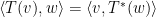


How is 


-
where
is an orthonormal basis for
.
This result tells the relation between the matrix representations of
- If
, then
is symmetric.
Below we shall see that self-adjoint operator
Recall that for linear operators on vector spaces, we study the concept of similarity and diagonalization: let us review a few important points below. By definition, “


- If
is a linear operator on vector space (not necessarily inner product space), then
is similar to
for any ordered bases
and
.
- If
Next suppose 


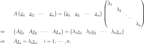
That means 


Furthermore, we can present the above result in the setting of linear transformation: Suppose 


![{\mathcal{E}=[\underline{x}_1,\cdots, \underline{x}_n]}](https://s0.wp.com/latex.php?latex=%7B%5Cmathcal%7BE%7D%3D%5B%5Cunderline%7Bx%7D_1%2C%5Ccdots%2C+%5Cunderline%7Bx%7D_n%5D%7D&bg=ffffff&fg=000000&s=0&c=20201002)

is similar to a diagonal matrix  There exists a basis
  for such that
  is diagonal There exists a basis for such that
  ,
,  We can find a basis consisting of eigenvectors of for
Now we turn back to inner product spaces. If


In terms of matrices, this is equivalent to finding a set of orthonormal eigenvectors
Here we make a nice observation: if 


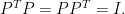
Such a matrix is called an orthogonal matrix (i.e. 


Hence for our problem 

Now we can state the following key result for self-adjoint linear operators (or in matrix setting, symmetric matrices):
Every
symmetric matrix
In the setting of linear operators, every self-adjoint operator
See also Lect28-29.pdf in the folder slides.

Leave a comment